In this article, I want to make the case for data-driven planning to describe the 7 key FP&A models that every organisation needs to plan, resource and monitor business performance.

Seven Key FP&A Models

Key planning questions

From a planning and review perspective, there are 7 key things that management needs to know about its business processes, each of which can be assessed in a range of analytical models:

• How efficient and effective are the organisation’s business processes? (Operational Activity Model)
• What trends are ‘hidden’ in detail? (Detailed History Model)
• What should long-range targets be set given where the market is heading? (Target Setting Model)
• Where is the organisation heading if it continues with its current business model? (Detailed Forecast Model)
• What could be done differently to better meet long-range targets, and how much would it cost? (Strategy Improvement Model)
• What choices/risks do management face, and what would be the impact on corporate goals? (Scenario / Optimisation Model)
• How much funding is required to implement the plan, and where will it come from? (Cash / Funding Model)

The models that answer each of these questions have different content and structures and are used by different people at different times. However, none can be omitted or ignored, and all need to operate as a single, data-driven management system.

From a planning systems point of view, this network of models can be visualised as follows:

 
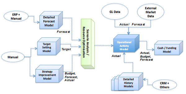
Schematic overview of the 7 key models required to manage performance

As can be seen, these models are fed with data from internal systems, such as the general ledger, and from external sources, such as market information, along with data supplied by end-users. Whether these models are separate entities will depend on the size and complexity of the organisation.  Some may be combined, while others may need additional supporting models to enable them to function effectively.  For now, we will consider them to be separate but linked models, which from a user view, operate as a single system. 

1. Operational Activity Model

The Operating Activity Model (OAM) is central to organisational planning that, as the name suggests, has a departmental activity focus.  Its purpose is to monitor business processes with a range of measures that allows management to evaluate their efficiency and effectiveness. In particular, it can be used to:

• Compare and contrast resources, workload and outputs both now and in the past
•  Assign budgets for ‘business as usual’, i.e. assuming that there are no strategic initiatives 

The model holds different versions of data, some of which flows from the other planning models.  These versions include:

• Target – contains the high-level goals set during the strategic planning process
• Budget – contains the allocation of resources for the current year/period.
• Forecast – contains the latest ‘best estimate’ of future performance for the next couple of months
• Actual – contains past results

The model is multi-dimensional in nature and uses ‘attributes’ that allow measures to be assigned to specific business process activities, and that categorises them as being:

• An Objective – these define what the organisation is trying to achieve in the long-term 
• A Business Process Goal – this measures the success of the organisation’s core business processes and support activities that directly lead to the achievement of objectives
• An Assumption - these monitor key assumptions made about the prevailing and forecast business environment that relate to the value set for the Business Process Goals
• A Work measure – these describe the volume (and sometimes the quality) of work performed by a particular department.   e.g. the number of mailings sent out by the marketing department as part of its lead-generation process
• An Outcome measure – this measures what an activity should directly achieve, e.g. the number of people that respond to a mailing 
• A Resource measure – these track expenditure that flows out of the organisation.

By using these attributes, the model is able to display data by the department but in relation to activity, outcome and resources used.  Below is an example of the types of reports that can be produced. 

The first report shows the corporate objectives and business process goals for a selected period.  This contains a mixture of the outcome, work and resource measures for both the budget and actual performance, as well as for last year.  Icon indicators are used to display whether results are getting ‘better’ or ‘worse’ than a target. 

 
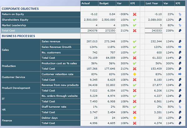
Sample report showing Corporate Objectives and how they are supported by business process goals.

The next report shows the outcome, work and resource measures for a selected department. As with the last report, actual performance is contrasted with the budget, while the end-of-year forecast is compared to the annual target.  From this, management can assess the relationship between workload and outcomes to judge whether the focus is on the right activities.

 
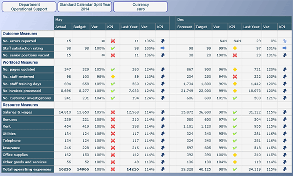
Sample report showing department work, outcome and resource usage

By using attributes as a filter, the above report is able to automatically display the appropriate measures as they apply to the selected department.  

These two reports just touch the surface of what can be displayed from the OAM.  Interestingly, most organisations have much of this data already, although it is typically shown in separate budgeting and scorecard/dashboard reports without making a connection between them. When treated in this way, the data can’t be used to model organisational value, and so much of its worth is lost.

2. Cash / Funding Model (CFM)

Closely linked to the OAM is the cash/funding model (CFM) that is used to assess the organisation’s need for financial resources. Some of those resources will be used to support operating expenses, and others will be required for capital investment or strategic initiatives. This model is linked to the operational activity model (OAM), which contains budgets and forecasts in order to predict future cash flows. It then goes on to help management assess the best source for any cash shortfalls.

Although it is true that most internal financial systems hold data relating to the flow of cash, what they do not allow is for management to model the data from a planning point of view.  For example:

• to see a revised cash flow based on new supplier credit terms or a change to customer payment profiles; 
• to consider the cost of funding an increase in production capacity to meet the projected demand for new products; or 
• to assess the impact on resources by outsourcing a particular function.

Similarly, financial systems do not hold the key assumptions that affect cash flow. For instance, inflation has a major impact on cash resources, yet the underlying data supporting any inflation assumptions is not contained within those systems.

Modelling cash flows and balances require different sets of information, as shown below:

 
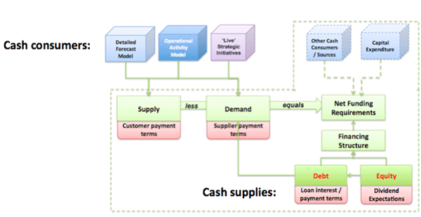
                               Cash / Funding model content

The dotted line indicates information stored within the CFM, while the bold lines indicate the data flows from other models in the planning framework. Data held can be summarised as follows:

• Customer and supplier payment terms. The CFM contains details about each major supplier and customer where the cash flow effect is to be calculated. Depending on how payment terms are defined (for example, in weeks or months), the time intervals in this model may be at a shorter increment than that of the OAM.
• Cash supply. Cash is modelled for budgets and forecasts. The supply side of cash is taken from the OAM, where the level of detail allows individual supplier or customer movements to be identified so they can match up with the appropriate customer details.
• Cash demand. Similarly, the demand side for cash is also taken from the OAM and takes into account all operational expenses, which for a manufacturer would include the supply of raw materials and manufacturing costs. It also includes any cash flows that arise in relation to capital expenditure. As with supply, these outflows are at a level where they can be linked to the payment profiles held within the CFM. 
• Net funding requirements. Rules within the CFM are used to ‘time-shift’ the imported cash supply and demand data into the time periods in which cash will flow in and out of the organisation’s treasury bank account(s).  To this, other cash consumers and income streams not covered are added. This may include items such as interest payments and dividend accruals. These details are entered directly into the CFM. By subtracting the demand for cash from the supply, management can review the financial resources required.

To address any cash shortfall, or to reduce the number of borrowings, budget and forecast data within the OAM can be reassessed to see which activities could be changed. The model also allows management to gauge the impact of changing customer and supplier payment terms. Assuming this has been done, the model can now be used to assess how any cash shortfall should be financed, with the two obvious financing sources being debt and equity.

When reporting actual results, much of the data within the cash flow model will be loaded directly from the underlying transaction systems, so there is little need for modelling other than to produce a comparison between budget and forecast versions.

3.  Detailed History Model (DHM)

The role of the Detailed History Model (DHM) is to back up the Operational Activity Model (OAM) described in the last blog when comparing actual results with the budget. The DHM has a much lower level of detail than the OAM and supports investigations into past performance. This will almost certainly include income and resources, as these will be made up of transactions held within the general ledger. Some of the workload and outcome measures may also have further details, which can be used to analyse business process activity.

There is likely to be more than one DHM, with each focusing on a specific area of performance, such as revenue or production costs.  However, it is not desirable to create DHMs for every measure, as this could distract management from what is important. Instead, DHMs should be created for those measures whose values play a significant part in either directly resourcing or monitoring a business process.

When defining a DHM, the question should be asked, ‘What information do I need in order to understand the actual results being presented in the OAM?’  The answer determines the level of detail, the analyses that are required, and the type of history model that will meet those needs.

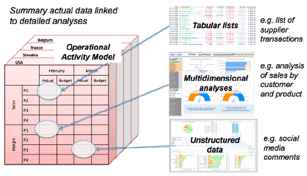
DHM’s can be of different model types that include: 

Transaction data set. These are tables of data that can be queried and summarised. An example of this type could contain the general ledger transactions behind each account code. These would be loaded from General Ledger (GL)  on a regular basis and could consist of the date, department, account code, supplier, and amount. Capabilities within the DHM would summarise this data by department, month, and account codes that are then fed into the appropriate place within the OAM.

The DHM could then be to support expense queries. For example, from a variance in the travel budget, a user would be able to drill down into the supporting DHM to see the transactions that made up the actual result. They could then issue another query that extracts transactions for a prior month to see if any expenses had been held over and hence had caused this month’s variance.
As with the other types of DHM, the ease of use and capabilities provided to an end user will depend on the technology solution being used. As a minimum, this type of DHM should support the following examples:

• Filters.  E.g. list all transactions making up a particular account code.
• Summaries. E.g. total all transactions for a particular account code and over a selected period.
• Sorting and ranking. E.g. show the top 10 departments as ranked by travel expenditure.

Multi-dimensional model. This type of DHM allows users to produce cross-tabular analyses. Data is stored and referred to by its business dimensions. Users then have free access to the way in which data is presented, which can incorporate charts, additional calculations, and colour-coded exceptions. Examples of this type of model include sales analyses that could include types of customers, products sold, discounts provided, returns, and shipping costs.
Unlike the transaction data set, a multi-dimensional model is able to provide the following:

• Multiple views of the data. E.g. show sales revenue by product and customer, customer profitability, and returns by product and location.
• Trends. E.g. calculate a rolling 12-month average and show this by month for the current year versus last year.
• Exceptions. E.g. show all customers whose year-on-year growth has been negative.

Unstructured data model. This final type of model provides support for non-numeric data, such as notes, news reports, social media discussions, and competitor product videos. By linking these into the OAM, qualitative information can be provided that can make a substantial difference in the way results are perceived.
For all the DHM types shown above, a security system is required that will automatically filter out data that the user is not allowed to see.

4. Detailed Forecast Model (DFM)

Detailed Forecast Models (DFM), like the DHM, are typically used in conjunction with the OAM to collect forecasts that operational managers believe they will achieve in the short term. This can include a range of measures, including workload, outcomes, and resources.

Although the OAM can collect forecasts at a summary level, there are measures that benefit from having this at a more detailed level. For example, revenue for a manufacturer can come from a range of customers and products, each of which has its individual profitability profile. As a result, the product mix can have huge implications on total revenue and costs. Therefore, predicting profitability with any degree of accuracy requires detailed knowledge of what is being sold, its volume, and to whom.

Similarly, sales of high-value items or those that relate to a project are often dependent on timing. In these cases, the sales process may be long, and when the business is won, the resultant impact on costs and revenues in a particular time period can be significant. Without knowledge of the detail, it is easy to jump to the conclusion that an over or underperformance is exceptional rather than expected.  For this reason, collecting information concerning the sales order pipeline and using this to populate the sales forecast improves not only accuracy but also provides insight should any variances occur.

As with DHMs, different measures can have a wide range of supporting detail and so there are likely to be multiple forecast models where each has a focus on a particular measure.  Again, not every measure warrants its own forecast model. Ideally, they are only created for measures where the underlying mix of detailed transactions can have a large impact on results when compared to plans.

 
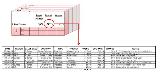
Providing detail behind a forecast so that informed assessments on accuracy can be made 

DFMs will typically hold just a forecast version of data, as actual results will be held in the detailed history model. (Remember, we are using the word model in a logical sense; the actual implementation may combine these into one physical model.)  For some measures, data may exist in another system (for example, many companies use SalesForce.com to collect sales information). If this is so, then the DFM may simply be a place where the latest data is stored that is then cleared out and repopulated each period. Alternatively, the DFM may be a system in its own right that is used to hold and track forecasts.

DFM’s can hold a range of data, not all of which is numeric.  For example, sales forecasts may include the following fields:

• Date that the sales forecast was entered
• Region responsible for the sale and where any revenue will be credited
• Sales executive involved
• Company being sold to
• Sales type (for example, whether the sale is to an existing customer or a new prospect)
• Product(s) being sold
• Value of the order
• Date contract is due to be signed and revenues recognised in the P&L summary
• Percent chance of the deal going ahead
•  Any notes to describe the current situation

As with DHM’s, data within a DFM can be sorted, summarised and reported. For example, show all sales due in the next three months ranked by the percentage chance of them being signed. This enables management to look in detail at a forecast so they can form their own opinion as to what could happen and take remedial action should they fall short of what is expected.

As an option, a sales DFM could apply the per cent chance measure to the value of each sales situation to produce a modified forecast value within the OAM, or the OAM could contain two measures—one holding a value that assumes all sales opportunities will materialise as held, and the other using the per cent chance. This provides a range of values that could be used to assess future performance.

It is also worth storing prior forecast versions so that, over time, a picture can be built up on the reliability of forecasts. For example, which salespeople are able to forecast with an accuracy of 5 per cent three months in advance? Which measures produce the most variability when viewed six months in advance? 

Knowing how trustworthy a forecast is can help determine which measures need regular inspection and the level of caution required when making decisions based on them.  Also, if managers are aware that forecasts are being monitored closely, then they are more likely to pay attention to the values they submit, which in turn are more likely to be trusted.

5. Target Setting Model (TSM)

The Target Setting Model (TSM) is a mathematical model that allows management to simulate different business environments as well as the way in which it conducts its business processes.  Its purpose is to generate target values that will challenge the organisation as to what its performance could be in the future.

The TSM typically relates the outcomes of organisational business processes (for example, products made, new customers acquired, and customers supported) to long-term objectives and resources. In many ways, it is similar to the Operational Activity Model (OAM) described in blog 3, except its rules are used to generate targets from a range of base data. This is also known as driver-based modelling. In effect, there are a few independent variables, such as forecasted unit sales volume, which are driven by dependent variables (e.g. price, material unit cost), which are based on assumptions about the business environment (e.g. market size and growth).

Measures for these models can be selected by taking long-range targets and determining what drives their value.  The answers to these are then subject to the same question and so on until a base ‘driver’ is encountered, i.e. a measure whose value determines the targets it supports.

More sophisticated models recognise constraints, such as production volumes, the impact of discounts, late delivery penalties, or that more staff will be needed at certain levels of sales. They also recognise that there is nearly always a time lag between the driver and the result it creates. 

It should also be noted that these models only work for those measures that can be directly related to drivers, such as costs and revenues. Other data, such as overheads, will still need to be included to produce a full P&L summary.

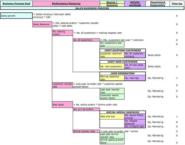
Sample relationship map on what drives sales growth.  Measures on the right-hand side are drivers.

Because of their simplistic nature, driver-based models are not able to take into account unpredictable external influences, such as unexpected market growth or changes in government legislation that impact taxes. This is where versions come into play. To see the impact of uncontrollable influences, the TSM is set up to hold a variety of scenarios where management can re-run the calculations with different driver values that simulate changing assumptions. For example, the model can be run with different sales conversion rates or unit costs, each of which will generate a new version of the P&L summary. These can then be displayed side-by-side, so management can see the impact of each change. 

The aim in doing this is to allow a range of options to be evaluated concerning the future. These options will revolve around business drivers, which, if based on business process outcomes, will cause management to rethink how these are conducted and what could be improved. The end result of the TSM is a scenario that management believes will give them the best outcomes for the available resources. These values are then used to set top-down targets within the OAM that can be referenced by individual departments during the budget process.

6. Strategy Improvement Model (SIM)

The Strategy  Improvement Model (SIM) is used to evaluate how the current performance of an organisation as forecast in the OAM (‘business as usual’) can be transformed into one that supports the targets set by the TSM. The model allows managers to propose initiatives that can then be assessed, approved or rejected for implementation. Initiatives could involve improvements to current operations, such as replacing old machinery, or something entirely new, such as developing a new range of services or entering new geographic markets. In both cases, initiatives typically represent a set of activities that are not part of current business processes. 

From a logical point of view, the SIM consists of two sets of data linked to the OAM, where ‘business as usual’ is kept.
 
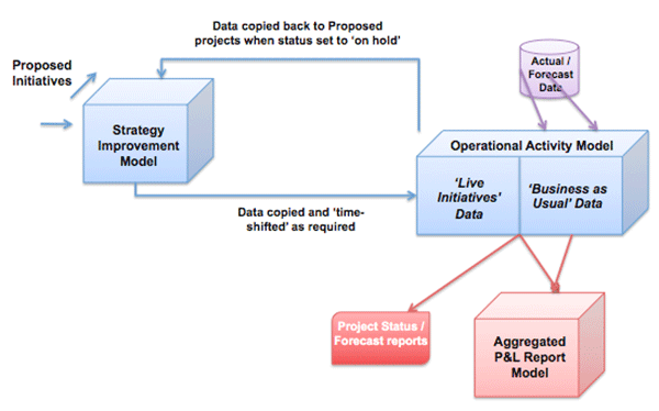
Relationship between initiatives and ‘business as usual’

The first part of the model is where managers propose initiatives that are linked to business process goals, departmental structures, and resources. Here initiatives can be reviewed, assessed, and gain approval.
When an approved initiative becomes ‘live’, its set of activities and associated data are transferred into the OAM, where it is kept separate from existing operational data. However, the OAM allows the accumulation of resources and other measures to give a total ‘business as usual’ plus ‘strategic initiatives’ position.

This is achieved by defining a new dimension in the OAM for strategy, which is made up of the following members:

Total strategy. This is a consolidation member that accumulates ‘business as usual’ data with ‘total initiatives’ data.

    - Business as usual. This member contains all of the data for current business processes but without applying any strategic initiatives.
    - Total initiatives. This is a consolidation member that contains the accumulation of data from its members; that is, the individual initiatives.

• Initiative 1. This contains the data for a selected initiative as transferred from the SIM.
• Initiative 2. This contains the data for a second selected initiative, and so on.

Keeping initiatives separate allows them to be monitored individually so management can keep a watchful eye on their implementation and resource usage versus expected benefits. Too often, initiatives are assumed to be responsible for an improvement in performance when no attempt has ever been made to actually measure whether this was true or whether the costs involved were worthwhile.
Linking the SIM to the OAM helps organisations to:

• Accurately define ‘business as usual’ (or baseline) performance of the current organisational business processes.
• Capture plan versus the actual cost of strategy implementation and the benefits being realised.
• Provide a transparent way of assessing priorities in the areas where performance improvement is most needed.
• Avoid vague claims or estimates for initiatives, as the SIM requires clarity.

As time passes, it should be possible to re-plan, suspend, delete, or select new initiatives as required. Should an initiative be suspended, it can be moved back to the SIM until required at a later date.

7. Scenario / Optimisation Model (SOM)

The last model in the planning framework is associated with Risk Management and enables managers to assess the impact of unexpected change and how it impacts corporate goals.  In the book ‘Best Practices in Planning and Performance Management’, author David Axson comments that  “Planning is not about developing a singular view of the future:  one of the most valuable elements of any planning activity is the ability to factor in the impact of risk on assumptions, initiatives and targeted results.”  He went on to say, “A scenario is a story that describes a possible future.  It identifies significant events, the main actors and their motivations, and it conveys how the world functions.”

As with DHM and DFMs, there may be more than one SOM.  For example, when balancing manufacturing costs with sales forecasts, some organisation’s employ sophisticated production models that determine which machines should produce which products and, as a result, what materials need to be ordered.

Similarly, when looking at the impact of a rise in commodity prices, it would be beneficial to assess a range of price values and to then compare the cost outcomes that these would generate.  From this, management can then decide how they would respond. For example, they may want to evaluate changing the current business structure or implementing a new initiative.

The aim of the SOM is to allow management to ‘play’ around with different scenarios, each of which is documented as to the assumptions made about the future business environment and the change that could be made in response.  These are presented back as a ‘side-by-side’ comparison from which decisions on the value set by the TSM can be evaluated or what adjustments may be required to the current budget in order to keep the original plan on track.