 Many sophisticated business environments use budgets as a bridge between actual and forecast. Within the corporate finance domain, budgets are used to allocate resources and provide a starting point for current and future period estimates. Budgets and revised budgets are often communicated to shareholders and the investor community in numerous ways such as earnings estimates and road show presentations in the form of a “current estimate”. The budget becomes a foundation for expectation.
Here are five key approaches to a sound budget model:
- Utilize Quantitative Forecast Techniques
- Integrate Statements
- Roll the Budget - Period to Period and Model to Model
- Distinguish Between Assets in Place and Growth
- Use Expected Values
1. Common Quantitative Forecast Techniques
Budgeting and forecasting methods can be divided into two broad categories: qualitative and quantitative. Listed below are common quantitative forecast techniques for financial statement modeling.
- Time series change (price, for example)
- Causal relationships (cash and receivables as a % of sales)
- Naïve - Beginning balances equaling prior period ending balances or flat-lined (fixed assets, debt)

Qualitative techniques may be used to adjust quantitative forecast output, based upon subject matter expertise.
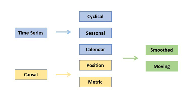
Time Series
A time series is simply a set of observations measured at successive points in time or over successive periods of time. Time series uses past trends of a variable.
- Cyclical. Any recurring sequence of points above and below the trend line that last more than a year is considered to constitute the cyclical component of the time series. Example; while the trend line for gross domestic product (GDP) is upward sloping, the output growth displays a cyclical behavior around the trend line.
- Seasonal. Seasonal components capture the regular pattern of variability in the time series within one-year periods. Many economic variables display seasonal patterns. Seasonal will require you to forecast by quarter and/or month.
- Calendar. Similar to seasonal, but follows a calendar path, such as weeks or quarters (Q1, Q2, Q3, Q4).
Causal
With causal relationships, the forecaster examines the cause-and-effect relationships of a variable with other relevant variables such as the level of consumer confidence, an income statement or balance sheet item. Below are examples of common causal relation calculations:
1. Position calculations represent a company's financial position regarding earnings, cash flow, assets or capitalization. Calculations can be expressed as a dollar amount, a percentage, or a comparison. Position calculations are often referred to as “common-sized” when it is uniformly applied to a whole statement.
- Cash % Assets
- Debt / Equity
2. Metric calculations assess financial position relative to a non-financial figure such as days, transactions or number of customers.
- Transaction Figures (Units Sold Per Day, Transaction Days, etc.)
- Utilization %
A widely-known causal method is regression analysis, a technique used to develop a mathematical model showing how a set of variables are related. Regression analysis that employs one dependent variable and approximates the relationship between these two by a straight line is called a simple linear regression. Regression analysis that uses two or more independent variables to forecast values of the dependent variable is called a multiple regression analysis.
Smoothing
Smoothing methods are appropriate when a time series displays no significant effects of trend, cyclical, or seasonal components (often called a stable time series). In such a case, the goal is to smooth out the irregular component of the time series by using an averaging process.
This relates closely to valuation’s use of “normalized” statements. The purpose of normalizing financial statements is to adjust the financial statements of a business to more closely reflect its true economic financial position and value conclusions of operation on a historical and current basis.
Moving
The term "moving" refers to the way averages are calculated—the forecaster moves up or down the time series to pick observations to calculate using an average of a fixed number of observations.
In calculating moving averages to generate forecasts, the forecaster may experiment with different-length moving averages. The forecaster will choose the length that yields the highest accuracy for the forecasts generated. Weights may be assigned to time periods.
Stochastic Modeling
Stochastic modeling is a statistical process incorporating a random element to a figure’s composition, based upon pre-determined parameter estimates. It can be used to determine revenue and expense items. This is one technique coined “predictive analytics”.
2. Integrate Statements
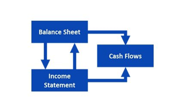
Integrated statements are a fundamental requirement for forecast DCF and the budget plays a part in that development process. Both conceptually and mechanically, integrated statements, by acknowledging the balance sheet-income statement-cash flow interdependency, demonstrate a core understanding of corporate finance synthesis and provide a foundation for both accounting and modeling structure. This is why the investment banks and Big Four consulting firms go to great lengths to develop this skill in their incoming analysts. Without integrated statements forecast, DCFs are likely to not hold upon to scrutiny.
Integrated statements can create circular references such as this:
- Interest expense on the income statement is a function of an average debt balance on the balance sheet.
- Current net income is dependent upon interest expense.
- Balance sheet equity is dependent upon current period net income.
- Debt is dependent upon total capitalization
- Total capitalization is dependent upon equity.
Though conceptually correct, both modeling organizations FAST and Best Practice Modeling recommend avoiding circularity. This can be solved by using a goal seek macro, for instance, maintaining a debt to equity level through all model periods. However this is handled, the best integrating approach will reflect the actual management approach employed in the organization.

3. Roll the Budget Downstream – Period to Period and Model to Model
The mechanics of the budget as the bridge between actual and future estimate are straight forward.
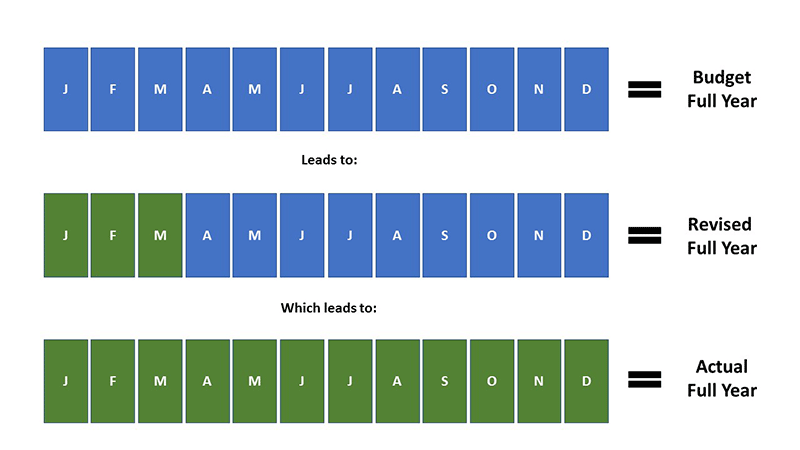
- With the budget in place, as actual data becomes available it replaces former budget data for the same period. The model’s number of periods (actual + forecast) does not change. Implied here is that the budget is developed from the same chart of accounts as actual. Revisions could be daily, weekly, monthly or quarterly.
- Future periods beyond the budget are impacted and a new, longer term plan is developed. This is because financial statements are impacted by time series movement and causal relation. The future is largely a result of past and current positions.
Therefore; actual, budget, current estimate and longer range plans are each dependent upon a respective upstream model. Any change to a prior period assumption or data may impact all future periods and models thereafter.

The granularity of the budget and a resulting downstream longer term plan is dependent upon need and ability. It is easier to begin by developing greater granularity in a model and rolling up into longer periods than it is to break apart a period into smaller segments, such as going from quarterly to monthly. Pay attention to this during development and attempt to anticipate future requirements.

4. Distinguish Between Assets in Place and Growth Opportunities
“Return on Capital (ROC), Return on Invested Capital (ROIC) and Return on Equity (ROE): Measurement and Implications” by Aswath Damodaran, illustrates well the power behind distinguishing between assets in place and growth assets. Separating the two allows management to more accurately gauge the following (quoting Damodaran):
-
How good are the firm’s existing investments? In other words, do they generate returns that exceed the cost of funding them?
- What do we expect the excess returns to look like on future investments?
This approach has numerous advantages. First, it eliminates noise and confusion. Second, it sets FP&A up for developing appropriate discount rates by project and growth opportunity, thus avoiding a one size fits all weighted cost of capital approach. And third, it acknowledges that future returns may not be the same as prior returns – discount rates change through time.

5. Use Expected Values
Though asset capacity and elasticity constraints (utilization rates) usually prevent the symmetrical distribution of outcomes from occurring in real life, as a planning and forecast tool, budgets most often assume a bell-shaped curve. In such a symmetrical distribution, the most likely outcome is equal to the probability weighted outcome. This will provide compatibility to most downstream models such as valuation models which most often are built upon the assumption of expected, as in valuation.
There is much discussion centered on the development, use, and validity of budgets. Viewing the budget as a bridge from past to future should help eliminate doubts, will provide commonality between FP&A models and synthesize FP&A responsibilities.
It all works together.
Rob Trippe is a financial modelling veteran. With over fifteen years’ experience, Rob has developed corporate finance models for valuation, M&A, forecasting and performance monitoring. He is widely respected for his deep understanding of corporate finance theory, lectures at university and has worked with some of the world’s largest and most respected firms. His research while at the investment bank Houlihan Lokey Howard & Zukin has been published in the Wall Street Journal and USA Today. His cash flow model work has been published in SEC and quarterly press release filings. Rob was accredited in valuation in 2008 and holds an MBA ,Finance from Boston College.
Subscribe to
FP&A Trends Digest

We will regularly update you on the latest trends and developments in FP&A. Take the opportunity to have articles written by finance thought leaders delivered directly to your inbox; watch compelling webinars; connect with like-minded professionals; and become a part of our global community.

